Neural Network from scratch - Part I

Humans have been obsessed with the idea of a machine doing things for them, or at least make their life easier for them, for a very long time now. Starting right from the invention of Wheel to the invention of Computer we pushed the limits of our brain to build such amazing objects. But something changed at the invention of computer, we realised that computers are far too good in one particular aspect as compared to humans, Calculations!

Then the human obsession of beating the computers at their own game began. We had some truly great human minds who not only challenged but won against the computer, may it be Shakuntala Devi beating the computer in finding the 23rd root of a 50 digit number or GM Garry Kasparov beating IBM’s Deep Blue in chess match. But soon we came to realise that computers(given correct configurations) are truly unbeatable at all the things that we previously won against them. So our focus shifted towards making use of the computers’ calculative capabilities to solve problems which we found difficult.

While this was happening though, some scientists were working on generating a mathematical model that would “learn”. The inspiration of that coming from the most perfect object that we knew, which already learnt and developed was, a Brain. Thus combining the power of huge calculations and the mathematical models that could learn, the idea of a Neural Network(Multi Layered Perceptron) was born.

What is a Neural Network?

Neural Networks are basically an attempt to make a mathematical model of the brain.

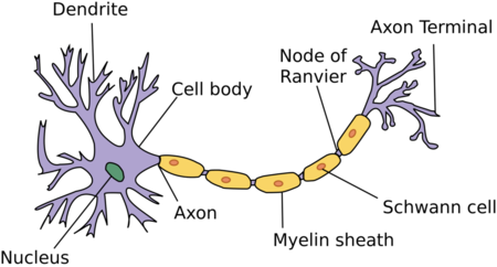A Biological neuron

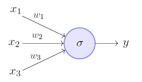A Perceptron

You can see the similarities between the biological and artificial structures. The fact that one of our brain’s components is an inspiration is pretty interesting, but I find it much easier to see a perceptron as a mathematical function that maps given input with a desired output

Let us see the working of a single neuron, the input values \(x_1\), \(x_2\), \(x_3\), multiplied by some weights \(w_1\), \(w_2\), \(w_3\), are passed into some function \(\sigma\) and value of output is

\(y = \sigma(x_1 \times w_1 + x_2 \times w_2 + x_3 \times w_3)\).

We call this “single layered” structure a Perceptron. But I must admit here that I have grossly oversimplified this whole process of neural network flow and even though the basic idea remains the same, there are multiple components and steps involved in the working of a neural network.

So without further adieu let us dive into the basics of Neural Network Architecture.

TOP

Architecture of a Neural Network

Let’s start small, as we saw in the above diagram, there’s an “input layer”, a “function layer” and a “output layer”, with funtion layer and output layer containing only single neuron. This structure is called a perceptron. If we were to extrapolate this idea and increase the number of neurons in each layer and the number of “function” layers we get a MLP(Multi Layered Perceptron), the structure would look something like this:

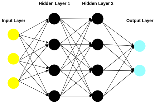
In the above architecture, there are four layers -

• 1 Input Layer with 3 neurons
• 2 Hidden(Function) Layers with 4 neurons each
• 1 Output Layer with 2 neurons

Components in architecture of a Neural Network

Neuron - A neuron is the most basic unit of a Neural Network. Each neuron stores information either as a real number or a mathematical operation that takes input, multiplies it by it’s weights and then passes the sum through the activation function to the other neurons.

Layer - A layer is multiple neurons working together. Input Layer takes in the data in form of vectors. Hidden layer processes that data using functions which we call activation functions. Output layer gives us the final result after the data has passed through the whole architecture.

Theoretically there is no restriction on the number of neurons in each layer or the number of layers, but in practice there is an upper limit to these numbers. What is this limit depends on the processing power of the system, latency limit and of course the cost of the financial cost of the system that would perform such calculations.

Workflow of a neural network

TOP

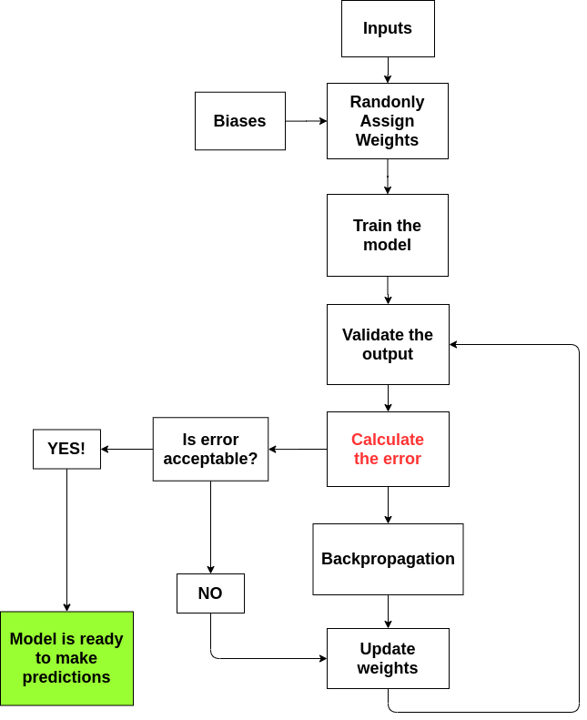
Components of a Neural Network flow

To save myself from the confusion I divided the whole process of a neural network training into 5 parts:

• Input Matrix
• Weights, Bias and Activation functions
• Feedforward process
• Loss Calculation
• Backpropagation

Input Matrix

The main idea of a neural network is to be able to solve our problems and there is no shortage of the problems that can be solved, may it be classification or regression or unsupervised learning. But here’s where it gets a little tricky, all the operations that we do are mathematical in nature and we won’t always get the data which is numerical, for example text data, what do we do in that case?

Well, let’s take a simple example we have to classify fruits with features as colour, taste, mass and two types of fruits(classes) Apple and Orange. Now mass is a numerical value, shouldn’t be a problem when it passes through the NN. However colour and taste are text values, but there is a simple way out here, since meanings of the words red and orange are not required but only the value that they posses we can simply index them({“red”:0, “orange”:1}) and use those numbers as inputs for NN. Same goes for the feature taste.

However things don’t remain that simple when meanings of the words matter, example say we are building a model which will classify the given sentence as positive or negative. In that case, simply assigning a number to each word won’t help since the number of unique words can be in millions!

I will be covering the concepts of NLP and how we would solve this problem, in depth, in future blogs. For now it is enough to know that we vectorize the words or sentences and number of neurons in input layer is same as the dimension of the word or sentence vectors.

Weights, Bias and Activation functions

• Weights decide the importance of the input coming into a neuron. Weights are initialised randomly in the beginning, later however they are automatically calculated based on the output. The weights are matrices which transform the input shape into the output shape by some mathematical operation(Matrix Multiplication in terms of Linear Algebra).

• Bias is a non-zero number defined by us and it acts the same way as \(c\) does in the equation \(y = m\times x + c\). Consider function \(f(x) = max(0,x)\) applied on the inputs \(x_1\) and \(x_2\) then if both \(x_1 = 0\) and \(x_2 = 0\) the function \(f(x_1 \times w_1 + x_2 \times w_2)\), will give us the output zero and for all of further process the values will keep getting multiplied by \(0\). To avoid this catastrophe we add a small non-zero value to the linear combination of weighted inputs.

• Activation Functions determines the output of each element (perceptron or neuron) in the neural network. Each neuron’s output is the input of the neurons in the next layer of the network, so the inputs pass through multiple activation functions until the output layer gives a prediction. There are various types of activation functions like ReLU(Rectified Linear Unit), Sigmoid, Tanh etc. basic definitions for which are mentioned in the Glossary. An important aspect of activation functions is that they must be computationally efficient because they are calculated across thousands or even millions of neurons for each data sample. During backpropagation, there is an increased computational strain on the activation function, and its derivative function. Neural networks rely on nonlinearity of activation functions, since real world problems are rarely linear!

Feedforward process

Forward propagation is a process of feeding input values to the neural network and getting an output which we call predicted value. When we feed the input values to the neural network’s first layer, it goes without any operations. Second layer takes values from first layer and applies multiplication, addition and activation operations and passes this value to the next layer. Same process repeats for subsequent layers and finally we get an output value from the last layer.

Loss Calculation

To calculate the gap between predicted value and actual value, we use Loss Function. So essentially, it calculates the error value. When used on the entire training set, we use Cost Function which is the average of loss functions of the entire training set. There are multiple variants of loss functions which can be used, MSE(Mean Squared Error), RMSE(Root Mean Squared Error), Log Loss etc.

Backpropagation

So far we have seen how we move through the neural network in the forward direction(left to right). Here after getting the output we find the error using a loss function. Now the question is how to reduce this error?

We do not have control over the input data that comes to us, but what determines the value of output is the weight we give to each value. So, if we were to find a way to change these weights so that the error reduces, our job will be done. Now, since this error is represented in the form a function, there’s a very nice mathematical way to find the minimum value this function can attain. That is finding local minima of the function i.e. given a function \(f\) finding the value of \(x\) for which \(f'(x) = 0\) or in more geometric terms finding value of \(x\) for which slope of \(f(x)\) is zero.

We call these derivatives, gradients and use these gradient values to calculate the gradients of the second last layer. We repeat this process until we get gradients for each and every weight in our neural network. Then we subtract this gradient value from the weight value to reduce the error value. In this way we move closer down to the Local Minima.

TOP

Conclusion

For nearly each of these components of a Neural Network there are variants, but to avoid creating confusion and making this post too long I have made a glossary of terminologies and their basic definitions which I will keep updating with every blog post. This was Part I of the Neural Network from Scratch series, in Part II we will go through the flow of NN using a real example and see how dimensions of matrices involved play a vital role. We will also see how to write all the above mentioned components using only python and then using Tensorflow library.

References

• Deep Learning Book by Ian Goodfellow, Yoshua Bengio and Aaron Courville

• Deep Learning Resources on Sebastian Raschka’s website

• Hackernoon’s this amazing blog post

• Neural Networks series by Grant Sanderson

TOP